Chapter 4 BigQuery

If you have a GCP project set up and are working with large volumes of structured data, you may have already uploaded this data to Cloud Storage or are just getting started. One robust use case for Google Cloud Storage (GCS) is its integration with BigQuery, Google’s serverless data warehouse designed to handle big data at scale.

If you’re familiar with R but have not used BigQuery before, there is no need to worry—you do not have to be an expert. For large datasets, a great workflow is to upload your data directly to BigQuery (either from your machine or from GCS) and then query it directly in R when needed. This approach allows you to take advantage of BigQuery’s performance and scalability without managing infrastructure or dealing with memory limitations in R.

This chapter will introduce you to BigQuery and explain its key concepts and terminology. You will also get an overview of the main functions and syntax used when working with BigQuery. Finally, we’ll guide you on connecting R to BigQuery, enabling you to query your large datasets seamlessly without requiring deep expertise in BigQuery.

4.1 Definition

BigQuery is Google’s fully managed, serverless data warehouse that enables scalable analysis over petabytes of data and is hosted on Google Cloud Platform. It is a Platform as a Service that supports querying using SQL syntax. It is the best location to store structured datasets of all sizes and is the recommended database for analytical use within DfT.

Some of the advantages of Google BigQuery are:

It is fully managed so there is no need for lengthy setup times or requiring any administration. Simply get access to a GCP project with access to BigQuery, and you are free to go.
It is serverless, both in terms of storage, so there’s no requirement to set up new disks or provision new database servers, and in terms of compute, so that you can query and transform petabytes of data with simple SQL code.

We offer training in BigQuery including:

Introduction to SQL in BigQuery

For users with no knowledge of SQL
BigQuery for SQL Users

For confident SQL users

4.2 How to: Access BigQuery

To get started with BigQuery, you will need access to a GCP project with BigQuery enabled.

To check your project has BigQuery enabled, go to the Google Cloud Console, and in the navigation menu on the left, look for BigQuery or use the search bar. If you can see and access it, BigQuery is enabled. If not, you may need to enable the BigQuery API from the API & Services panel.

Once inside the BigQuery interface, you’ll be taken to the BigQuery Editor. This is where you can run queries, view your datasets, and manage your tables. Here’s an overview of what you’ll see and some key terms.

4.2.1 BigQuery interface

The interface is split into two main panels:

This is where you see your GCP project(s), datasets and tables. You can also pin other projects you have access to by clicking “Add Data” and selecting “Pin a Project”.

Additionally, you can create a new GitHub repository or connect to an existing one from here; however, this is a more complex process that involves additional setup.

The central part of the screen is the SQL workspace where you can write, run, and save SQL queries. When you run a query, the results appear in the panel just below the editor.

4.2.2 BigQuery editor

The BigQuery Editor includes several helpful features designed to make working with your data easier:

Syntax Highlighting and Error Checking

SQL keywords are colour-coded for better readability. As you type, the editor checks for errors, such as incorrect column names or syntax issues, and provides suggestions or corrections.

Auto-complete

The editor provides real-time suggestions based on your schema and previous queries, helping you write accurate code faster.

Query History

You can view all past queries you’ve run from your current session. This makes it easy to revisit, tweak, or rerun previous code.

Visual Query Builder

For those less comfortable writing SQL from scratch, BigQuery offers a visual tool that lets you drag and drop tables and columns to build your query logic.

Formatter and Validator

The editor can automatically format messy SQL code and validate queries before you run them—useful for catching issues early.

Estimated Query Cost

BigQuery will tell you how much data your query is going to scan before you hit run, helping you manage costs more effectively.

4.2.3 Terminology

Here are some terms you’ll come across frequently:

a Google Cloud Project: This top-level container holds all your GCP resources, including BigQuery. Each project has a unique ID linked to a billing account. Everything you do in BigQuery—creating datasets, storing tables, running queries—happens within a project
a Dataset: A dataset groups related tables and views that live inside a project. Think of it like a folder in a database system. Datasets help organise your data and allow you to set access permissions at a higher level
a Table: Tables store the actual data, which is organised into rows and columns. Each table has a schema (i.e., structure) that defines the column names, data types (e.g., STRING, INT64), and whether null values are allowed

Other terms that would be good to know include:

Schema: The definition of the structure of your table—this includes column names, data types (such as STRING, INTEGER, or TIMESTAMP), and whether each column can contain NULL values. You define the schema when creating or loading a table.
View: A virtual table defined by a saved SQL query. Views don’t store data—they run the query each time they are accessed, so the data is always up to date
Job: Every time you run a query, load data, export a table, or perform another task in BigQuery, it runs as a job. You can monitor job status, review history, and troubleshoot errors using the Job history tab in the BigQuery console.

In the next section, we will explore how to use SQL within BigQuery, connect BigQuery to R, and discuss which approach—using SQL directly in the web editor and bringing that data into R or querying BigQuery from within Cloud R—is best suited for reading data into your analysis environment.

4.3 How to: Use BigQuery

Whether you’re an advanced SQL user or primarily work in R, we will guide you through BigQuery syntax and highlight key differences and equivalents between them. But first, let’s ensure you have data uploaded and/or added to BigQuery.

So, we have seen how to transfer data from a GCS bucket into BigQuery—but what if you have extensive, structured data that you want to upload or add directly to BigQuery without storing it in Cloud Storage?

4.3.1 Create a Dataset and Table

Following the announcement of the GCP project transition, the “Creating a Dataset” click-point (ClickOps) option will be unavailable.

We have retained this method in the playbook because, although we are in the early stages of moving the GCP project to the new infrastructure, some existing projects may still utilise the “ClickOps” – but this will no longer be an option once the GCP project transition is complete.

This change only affects the “Creating a Dataset”. There is no change to how you create a BigQuery table — the process for creating tables will remain the same before, during, and after the transition.

Video tutorials:

Creating a dataset in BigQuery

Creating a table in BigQuery:

Written instructions:

Step 1: Open BigQuery in the Cloud Console

Navigate to the BigQuery Console and ensure you’ve selected the correct GCP project from the top project selector.

Step 2: Create a Dataset

In the left-hand Explorer panel, click the name of your project.
Click the “Create dataset” button.
Enter a Dataset ID (e.g., sales_data_2024).
Choose a data location (e.g., europe-west2) and optionally set a default table expiration or encryption settings.
Click “Create dataset”

Step 3: Create a Table

Click on the 3 vertical colons on the right of your newly created dataset
Click “Create table”
Choose how you want to add your data:

Upload a file
Create an empty table and define the schema manually
Link to an external table (e.g. Cloud Storage or Google Sheets)

Fill in table name, scheme details (e.g. column names, data types), and table options
Click “Create table”

4.3.2 Naming BigQuery Objects

4.3.2.1 Datasets

Be Descriptive

Use descriptive names that convey the purpose or content of the dataset. Avoid generic or ambiguous names.

Example: passenger_id instead of id.

Use Lowercase

Stick to lowercase letters to maintain consistency and readability.

Example: seat_number instead of SeatNumber.

Separate Words

If your dataset name consists of multiple words, separate them with underscores (_) for better readability.

Example: user_activity

4.3.2.2 Tables

Follow Dataset Convention

Ensure that table names within a dataset follow a consistent naming convention related to the dataset name.

Example: transactions for a table within the customer dataset.

Include Entity and Descriptor

Incorporate what the table contains along with a descriptor if needed.

Example: orders, customer_info, product_catalog etc

Use Descriptive Names

Like datasets, use descriptive names for tables that clearly represent the data they hold.

Example: sales_by_region, user_activity_logs etc.

Avoid Abbreviations

Minimise the use of abbreviations unless they are widely understood or significantly reduce the length without compromising clarity.

Example: Prefer customer_information over cust_info.

Use Consistent Naming Style

Stick to a consistent naming style across all tables within your project to avoid confusion.

Example: If you’re using underscores to separate words (sales_data) in one table name, maintain this convention across all table names.

4.3.2.3 Views and procedures

Indicate Object Type

Prefix views and procedures with view_ or procedure_ to clearly distinguish them from tables.

Example: view_customer_summary

Maintain Naming Consistency

Apply the same naming conventions (e.g. snake_case, descriptive names) to views and procedures as you do for tables. This ensures your datasets remain clean, navigable, and maintainable.

4.3.2.4 Avoid these in naming BQ objects

Special Characters and Identifier Rules

Special Characters: BigQuery distinguishes between unquoted and quoted identifiers.
- Unquoted Identifiers:
  - Must begin with a letter or an underscore (_).
  - Can only contain letters, numbers, and underscores.
  - Cannot contain spaces or special characters (e.g. !, @, #, $, ^, &, *, (, ), -, +).
- Quoted Identifiers:
  - Enclosed in backticks (`).
  - Can contain any characters, including spaces and symbols.
  - Must be quoted if using reserved keywords or unsupported characters.

Reserved Keywords

Avoid using SQL reserved words and functions (e.g., SELECT, FROM, WHERE, JOIN) as object names to prevent syntax errors or ambiguity.

Length Limitations

BigQuery object names can be up to 1,024 characters for datasets and tables. Views, procedures, and other object types may have shorter limits.

Unicode Characters

BigQuery supports Unicode characters in object names, but ensure they are readable and compatible across different systems and teams.

Start with Underscore

Although allowed, avoid starting object names with an underscore (_) as this is typically reserved for system-generated or special-use objects.

Numeric-Only Names

Avoid using names that consist only of digits. They can be unclear, ambiguous, or prone to misinterpretation.

Leading Digits

While BigQuery allows object names to start with numbers, it’s recommended to avoid this to reduce parsing issues or confusion.

Reserved Prefixes

Avoid using prefixes like bq_, sys_, or goog_, which may be reserved for internal or system use.

4.3.2.5 Miscellaneous

Document Naming Conventions

Document your naming conventions in a central location, such as a shared README or internal wiki. This helps ensure all team members understand and follow the same standards.

Keep Names Concise but Informative

Choose names that strike a balance between brevity and clarity. Avoid names that are too long or too generic—clarity should not come at the cost of readability.

Regularly Review and Update

Set aside time periodically to review and refine naming conventions. This ensures they remain relevant as your project scales or changes over time.

4.3.3 Querying using SQL

When working with large datasets in BigQuery, it is a good practice to filter, group and summarise your dataset using SQL before bringing it into R. This reduces the amount of data you need to transfer, saving disk space, RAM and processing time in R. And most importantly, saving your Cloud R server from crashing, disrupting not only your work but others too. In this section, we’ll cover the core SQL operations in BigQuery that will allow you to filter, aggregate, and reshape your data.

A full reference documentation of the Query syntax you can use for SQL queries.

SELECT and FROM

SELECT: Retrieve specified columns from a table or dataset
FROM: Specifies the table or dataset from which to retrieve information


SELECT column1, column2 
FROM `project_id.dataset_name.table_name`;

; is used as a statement terminator. It signals the end of an SQL statement and is often used when multiple SQL statements are written together in a script or query.

This specifies that data is being selected from the table table_name within the dataset dataset_name.

WHERE

Filter rows based on a condition. Only rows that meet the condition will be included in the result set.


SELECT * 
FROM `project_id.dataset_name.table_name`
WHERE column1 > 100;

This filters the rows where the value in column1 is greater than 100.

The * means “select all columns” – it will return every column in the table_name within the specified dataset and project.

CASE WHEN

Create new columns with values based on conditions. It acts like an if..else in SQL, assigning different outputs depending on the data in each row.


SELECT column1,
       CASE 
         WHEN column1 > 100 THEN 'High'
         WHEN column1 > 50 THEN 'Medium'
         ELSE 'Low'
       END AS category
FROM `project_id.dataset_name.table_name`;

This creates a new column called category.

The CASE statement must always end with END, which tells SQL that you’re finished defining the logic. The result of the CASE expression is then assigned as an alias using AS category, so it appears as a new column in the output.

AND / OR

AND or OR: Combine multiple conditions in the WHERE clause.


SELECT * 
FROM `project_id.dataset_name.table_name`
WHERE column1 > 25 AND column2 = 'XYZ';

This filters rows where column1 is greater than 25 and column2 is equal to ‘XYZ’. Both conditions must be true for a row to be included.

You can also use OR to include rows where either condition is true. For example:


SELECT * 
FROM `project_id.dataset_name.table_name`
WHERE column1 > 25 OR column2 = 'XYZ';

In that case, rows will be included if either condition is true.

JOIN

JOIN: Combines rows from two or more tables based on a related column between them (known as a join condition).
INNER JOIN: Returns only rows where there is a match in both tables.
LEFT JOIN: Returns all rows from the left table, and matching rows from the right table. If no match exists, NULL values are returned for columns from the right table.
RIGHT JOIN: Returns all rows from the right table, and matching rows from the left table. If no match exists, NULL values are returned for columns from the left table.
FULL OUTER JOIN: Returns all rows when there is a match in either table. If no match exists, NULL values are returned for the missing side.
CROSS JOIN: Returns the Cartesian product of both tables (all possible row combinations).


SELECT o.order_id, c.customer_name
FROM sales.orders o
LEFT JOIN sales.customers c
  ON o.customer_id = c.customer_id;

In this example:

o is an alias for the orders table.
c is an alias for the customers table.
The LEFT JOIN ensures all orders are returned, even if some customers do not have matching records.

CREATE TABLE

Used to create a new table.


CREATE TABLE `project_id.dataset_name.new_table_name` AS
SELECT column1, column2
FROM `project_id.dataset_name.existing_table_name`
WHERE column1 > 25 AND column2 = 'XYZ';

This syntax creates a new table at the specified location project_id.dataset_name.new_table_name.

The AS keyword populates the new table with the result of the SELECT query, which can filter and transform data.

This is useful for storing the results of a query in a new table for future use.

CREATE TEMP TABLE

Used to create a temporary table that exists only during the session or query execution.


CREATE TEMP TABLE temp_table AS
SELECT * 
FROM `project_id.dataset_name.table_name`
WHERE column2 = 'XYZ';

This creates a temporary table named temp_table that stores all rows where column2 equals ‘XYZ’.

Temporary tables are useful for breaking complex logic into smaller steps without creating permanent tables in your database.

WITH

WITH: Defines a Common Table Expression (CTE), which is a temporary, named result set that can be referenced within the main query.
CTE: Useful for breaking down complex queries into smaller steps, improving readability, and reusing logic multiple times in the same query.


WITH recent_orders AS (
  SELECT customer_id, order_id
  FROM sales.orders
  WHERE order_date >= '2024-01-01'
)
SELECT customer_id, COUNT(order_id) AS total_orders
FROM recent_orders
GROUP BY customer_id;

In this example:

recent_orders is a CTE that selects orders placed after January 2024.
The main query then references recent_orders instead of repeating the filtering logic.
This improves readability and makes the query easier to maintain.

GROUP BY

Groups rows that have the same values in specified columns into summary rows. It’s commonly used with aggregation functions like COUNT(), SUM(), or AVG().


SELECT column3, COUNT(*) AS count
FROM `project_id.dataset_name.table_name`
GROUP BY column3;

This groups the data by column3 and counts the number of occurrences in each group. The result will show one row per unique value in column3, along with how many times it appears.

HAVING

Filters results after the GROUP BY aggregation has been applied.


SELECT column3, AVG(column1) AS avg_column1
FROM `project_id.dataset_name.table_name`
GROUP BY column3
HAVING AVG(column1) > 50;

This filters the grouped results to only include rows where the average value of column1 is greater than 50.

HAVING is similar to WHERE, but it works on aggregated/grouped data.

LIMIT

Restricts the number of rows returned by the query.


SELECT * 
FROM `project_id.dataset_name.table_name`
LIMIT 100;

This limits the result set to only the first 100 rows. Useful when previewing large datasets.

ORDER BY

Sorts the query results by the specified column.


SELECT column1, column2
FROM `project_id.dataset_name.table_name`
WHERE condition
ORDER BY column1 ASC;

This sorts the results by column1. The default order is ASC (ascending). Use DESC to sort in descending order.

You can also sort by multiple columns if needed:


ORDER BY column1 ASC, column2 DESC;

4.3.4 Best practices for writing SQL in BigQuery

Writing SQL in a clear and consistent way makes your queries easier to read, share, and maintain. In BigQuery, where queries can get long and complex, adopting good style conventions ensures efficiency and collaboration across teams.

Naming Conventions

Use snake_case for all identifiers (tables, columns, aliases, Common Table Expressions (CTEs), and views).
- Good examples: customer_id, order_date
- Bad examples: CustomerID, OrderID
Be descriptive and explicit - names should describe what the column or table contains.
- Good examples: avg_order_value
- Bad examples: aov
Prefix helper tables or CTEs with context if necessary (e.g., sales_by_region).
Avoid reserved words (e.g., date, rank). If unavoidable, wrap in backticks.

Formatting and Spacing

Capitalise SQL keywords: SELECT, FROM, WHERE, JOIN.

Indent clauses consistently, with one clause per line:


SELECT
  customer_id,
  COUNT(order_id) AS total_orders
FROM
  sales.orders
WHERE
  order_date >= '2024-01-01'
GROUP BY
  customer_id
ORDER BY
  total_orders DESC

Align AS aliases when selecting many columns.
One column per line in SELECT for better readability and cleaner version control.

Table Aliases

A table alias is a short name you assign to a table for convenience. It makes queries shorter and easier to read, especially when you are joining multiple tables.

Example:


FROM sales.orders o

Here, o is an alias for sales.orders. You can then reference o.customer_id instead of typing the full table name every time.

Best practices for aliases:

Use short, intuitive aliases (e.g., o for orders, c for customers).
Be consistent – use the same alias for the same table across queries.
Avoid meaningless aliases like t1, t2.

Joins and Subqueries

Always use explicit join types (INNER JOIN, LEFT JOIN) rather than implicit joins.

Place join conditions on new lines for clarity:


FROM sales.orders o
LEFT JOIN sales.customers c
  ON o.customer_id = c.customer_id

Here:

o refers to the orders table (sales.orders).
c refers to the customers table (sales.customers).
The ON clause specifies how the two tables are linked.

Common Table Expressions (CTEs)

A CTE (Common Table Expression) is a temporary, named result set defined with a WITH clause. CTEs are especially useful in BigQuery for breaking down long queries into clear, logical steps.

Example without CTE


SELECT
    customer_id,
    COUNT(*) AS order_count
FROM (
    SELECT
        customer_id
    FROM
        sales.orders
    WHERE
        order_date >= '2024-01-01'
) sub
GROUP BY
    customer_id

Example with CTE


WITH recent_orders AS (
    SELECT
        customer_id
    FROM
        sales.orders
    WHERE
        order_date >= '2024-01-01'
)
SELECT
    customer_id,
    COUNT(*) AS order_count
FROM
    recent_orders
GROUP BY
    customer_id

Here, recent_orders is a CTE. It makes the query easier to read and maintain.

Benefits of CTEs

Improve readability by breaking logic into named steps.
Support reusability within a single query.
Make queries easier to debug and maintain.

Note: In BigQuery, CTEs don’t necessarily improve performance—they are re-expanded at runtime. Use them mainly for clarity.

Consistency

Use a standard clause order: SELECT → FROM → JOIN → WHERE → GROUP BY → HAVING → ORDER BY → LIMIT.
Be consistent with aliasing – always use AS, even though BigQuery allows you to omit it.
Standardise date and time functions (DATE(), PARSE_DATE(), FORMAT_DATE()).

Comments and Documentation

Use -- for inline comments. Place comments above logical sections.


-- Get total orders per customer since January 2024
SELECT
  customer_id,
  COUNT(order_id) AS total_orders
FROM
  sales.orders
WHERE
  order_date >= '2024-01-01'

Keep comments concise and focused on intent, not obvious details.

Performance considerations

Avoid SELECT * – only select the columns you need.
Filter early with WHERE or QUALIFY to minimise scanned data.
Use table partitioning and clustering effectively to optimise costs and speed.

4.3.5 Optimise your SQL Queries

Although BigQuery is a powerful tool within GCP for storing and analysing datasets of any size, writing efficient SQL queries is essential to fully leverage its performance.

Below are some tips for optimising BigQuery performance—particularly important when working with large datasets, where even small improvements can have a significant impact.

Avoid repeating subqueries

If a subquery needs to be used multiple times, it’s better practice to use Common Table Expressions (CTEs). Unlike subqueries, CTEs can be reused within the same query, simplifying complex queries and improving performance.

Use the Largest Table as a Base

Using the largest table as the base table in your query can improve performance in BigQuery.

The base table refers to the first table in a FROM clause or the one driving the query in a JOIN. The largest table is the one with the most rows or data volume being queried. Choosing it as the base allows BigQuery to optimize how the data is processed and joined.

Why it helps:

Improved parallelisation: BigQuery processes the largest table first and distributes the work more efficiently across compute nodes.
Columnar storage efficiency: When the largest table drives the query, BigQuery can better leverage its columnar format for filtering and selecting data.
Lower data processing costs: Starting with the largest table can reduce the need to scan multiple tables unnecessarily, especially if the other tables are smaller and filtered during joins.
Materialised view alignment: Helps when materialized views are used, as BigQuery can reuse precomputed data more effectively.
Better cache utilisation: BigQuery’s cache works at the table level, so using a frequently queried large table first can increase cache hit rates.

Avoid using SELECT *

Avoid using SELECT * for several reasons:

Transfers more data over the network, increasing latency and costs.
Processes and charges for more data than necessary.
Can impact query performance by fetching unnecessary columns.
Less likely to benefit from BigQuery’s caching mechanisms.
Makes queries less readable and more prone to errors with schema changes.

Use temporary tables for immediate results

Temporary tables are useful when you need to store intermediate query results that you don’t need to keep permanently. They are often quicker to create and discard, and they help keep your workspace organised.

Best practice: Use temporary tables when working with subsets of data or aggregations that are part of your analysis pipeline and discard them once you are done to save on storage costs.

Create tables for data you need to retain

When working with data that needs to be saved and reused for multiple analyses or projects, create permanent tables. This will help you avoid re-running complex queries every time you need the same data.

Best practice: Only create permanent tables for datasets that will be reused frequently and ensure that table names are clear and descriptive to make data retrieval easier.

Leverage table partitioning

Table partitioning organizes large datasets into more manageable sections, significantly improving time and cost efficiency when querying in BigQuery.

See our section on See the advanced section for more on partitioning.

Review data model and partitioned columns

In addition to partitioning, consider using clustering columns within partitions to organize data further. This can improve performance for queries with range-based filters.

Use parameters to filter on partitioned tables to enable partition pruning by the BigQuery engine, reducing the amount of data processed during queries.

See our section on See the advanced section for more on clustering.

Consider views for logic reuse without storing data

Unlike tables, views do not store data themselves. Instead, they store the SQL logic used to generate the data and run the query each time the view is accessed. Views are useful when you want to standardise business logic or simplify complex queries without duplicating data.

Best practice: Use views when the underlying data changes frequently or when you want to avoid maintaining duplicate datasets, but be mindful of performance since the query runs each time the view is queried.

Filter data before loading to BigQuery if dataset is too large

If your dataset in Cloud Storage is too large to load all at once, consider using a temporary external table in BigQuery. This lets you query and filter only the data you need before saving it as a permanent table.

Best practice:


CREATE OR REPLACE EXTERNAL TABLE my_dataset.temp_table
OPTIONS (
  format = 'CSV',
  uris = ['gs://your-bucket/your-file.csv']
);

-- Then filter and save the reduced data
CREATE OR REPLACE TABLE my_dataset.filtered_data AS
SELECT *
FROM my_dataset.temp_table
WHERE important_column IS NOT NULL;

CREATE OR REPLACE: This tells BigQuery to create the table if it doesn’t exist, or overwrite it if it already does.
EXTERNAL TABLE: This creates a temporary link to data that lives outside BigQuery — in this case, in Google Cloud Storage.
OPTIONS: This section specifies settings for the external table — including file format and location.
- format = 'CSV': Tells BigQuery that the file in Cloud Storage is in CSV format
- uris = ['gs://your-bucket/your-file.csv']: This points to the actual file in Google Cloud Storage. It uses the gs:// URI scheme, which stands for “Google Storage”. You can also include multiple files using wildcards like gs://your-bucket/folder/*.csv.

For best practices on designing effective tables in BigQuery, see our Effective Table Design section.

4.3.6 Saving your queries

It’s important to save your queries in BigQuery to keep track of the logic, share it with colleagues, and reuse it later. BigQuery provides several ways to save your work:

Save queries in the BigQuery editor

In the BigQuery Editor, you can save your SQL queries for future use. After writing your query, click the Save button and give your query a meaningful name. You can also save queries as “saved queries” in the BigQuery Console, which allows you to quickly run them again or share them with others.

Use named queries for reusability

Named queries are a great way to store reusable SQL queries. These are especially useful for complex queries that are frequently used across different projects or departments.

Best practice: Save commonly used queries as named queries for quick access and easy collaboration with your team.

Export query results to external storage

After executing a query, you can export the results to a file, such as CSV, JSON, or other formats, and store it in Google Cloud Storage. This helps when you need to share large datasets or move the data to other applications like Cloud R.

Best practice: Export results to Google Cloud Storage when the data needs to be shared or analysed in external tools and ensure that sensitive data is properly protected during the export process.

4.4 Effective Table Design

Designing an effective table schema — or data modeling — is crucial for maximising the benefits of BigQuery.

This section walks you through best practices and strategies for efficient table design in BigQuery, helping you fully harness its analytical power.

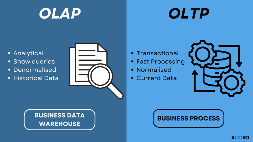
When it comes to databases, there are two primary systems designed to serve different purposes: OLTP (Online Transaction Processing) and OLAP (Online Analytical Processing).

4.4.1 OLTP: Online Transaction Processing

OLTP systems are used in traditional databases such as SQL Server. They are designed to efficiently manage transactional data, handling large volumes of short, atomic operations like inserts, updates, and deletes. OLTP systems prioritise data integrity and real-time performance.

Common OLTP use cases include:

E-commerce transmissions: Processing customer orders, payments, and inventory updates
Banking systems: Managing account balances, transfers, and customer transactions

4.4.2 OLAP: Online Analytical Processing

OLAP systems — such as BigQuery — are optimised for analysing and querying large volumes of data. They are designed for read-heavy operations, enabling complex queries and aggregations across extensive datasets to extract insights.

Typical OLAP use cases include:

Sales data analysis: Aggregating sales across regions, products, and time periods to identify trends
Customer behaviour analytics: Analysing large datasets to understand customer preferences, purchase patterns, and segmentation

Show image

4.4.3 The Shift towards Denormalisation and One Big Table (OBT)

Historically, data warehousing solutions — a common application of OLAP systems — have used schemas such as the STAR schema or snowflake schema. These approaches involve a degree of normalisation and organise data into fact tables and dimension tables, making queries more straightforward and efficient in traditional environments.

However, in the context of BigQuery, a different approach is often more effective.

Show image

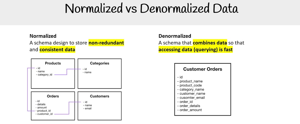
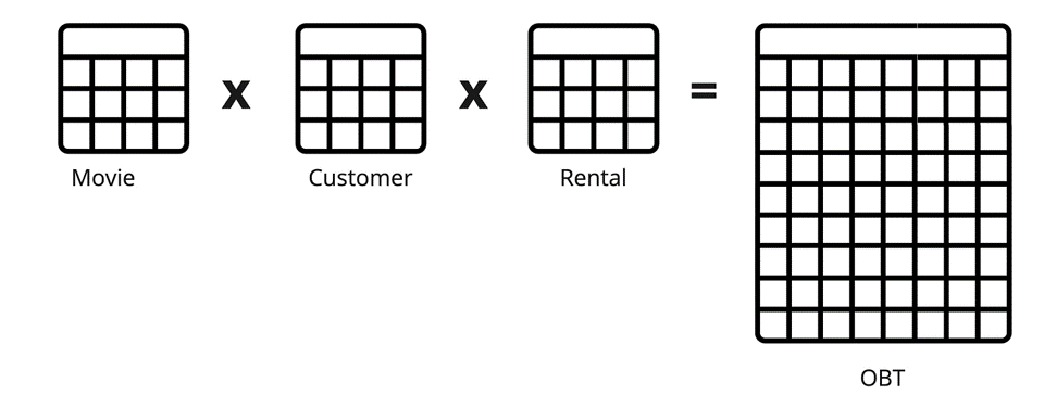
BigQuery, with its managed, serverless, and highly scalable architecture, is particularly well-suited to handling denormalised data — often referred to as the “One Big Table” (OBT) approach.

Denormalisation involves consolidating data into a single, wide table, which significantly simplifies queries by reducing or eliminating the need for joins. This approach works especially well in BigQuery, where:

scanning large datasets is fast,
costs are based on the volume of data processed, and
performance scales automatically with demand

By adopting denormalised structures, you can achieve faster query performance, simpler data models, and a more accessible experience for analysts working with the data.

Show image

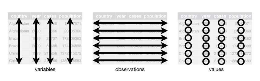
4.4.4 Adopting Tidy Data principles

When designing schemas for BigQuery, it’s beneficial to adopt tidy data principles. Tidy data complements the One Big Table (OBT) approach by ensuring that datasets are organised in a consistent and intuitive way:

Each variable forms a column
Each observation forms a row
Each type of observational unit forms a table

This structure enhances clarity and ease of use, enabling more efficient querying and analysis. Tidy data principles also support a straightforward mapping of data to analytical models and visualisation tools, helping to streamline the entire data analysis workflow.

Show image

4.4.5 Best practices

As a result of working with more traditional databases, many of our existing datasets are not optimally designed to take full advantage of BigQuery’s capabilities.

We will present three common practices that should be implemented to get the most out of our new tooling.

4.4.5.1 Best Practice 1: Long-Format Tables

Instead of spreading data across many columns, a more effective approach in BigQuery—aligned with tidy data principles—is to use long-format tables. This means having one column for the variable (e.g., “Hour”) and another for the value (e.g., “Value”), with each row representing a single observation. This format offers several advantages:

Simplifies queries: Queries become easier to write and understand, as you can filter by the variable column and aggregate over the values.
Improves scalability: As your dataset grows, you can simply add more rows instead of modifying the table schema.
Enhances performance: BigQuery is optimised for scanning large datasets and performs efficiently with long-format tables, especially when used with partitioning and clustering.

In the example below, we show two tables: the first in wide format, and the second in the desired long format.

Before Transformation (Wide-Format)

Date	Hour1	Hour2	Hour3	…	Hour24
2024-02-27	100	150	120	…	90

After Transformation (Long-Format)

Date	Hour	Value
2024-02-27	1	100
2024-02-27	2	150
2024-02-27	3	120
…	…	…
2024-02-27	24	90

4.4.5.2 Best Practice 2: Big Tables

Another common practice we’ve observed is splitting datasets into separate tables (e.g., one table per year). While this may have been a sensible approach in the past—particularly when limited by the processing power of SQL Server—a more efficient strategy in BigQuery is to consolidate all data into a single, large table, using a column to represent the dimension previously used to split the tables (e.g., “Year”). This approach plays to BigQuery’s strengths in handling large-scale datasets and offers several key benefits:

Centralises data management: Simplifies maintenance by reducing the number of tables.
Facilitates comprehensive analysis: Enables complex queries without requiring cross-table joins, allowing analysts to easily perform longitudinal and trend analyses.
Optimises query performance: When combined with partitioning (e.g., by “Year”), it reduces the volume of data scanned, which in turn lowers costs and improves execution time. (See our section on See the advanced section for more on partitioning.)

Note: While consolidating similar data across time (e.g., bus fares over multiple years) is recommended, unrelated datasets (like airport listings and bus fares) should not be combined into a single table. It’s important to keep datasets logically grouped and contextually relevant to their use case.

4.4.5.3 Best Practice 3: Use Meaningful Observations

The final practice we’ll discuss is a traditional database optimisation technique: substituting real values with integer codes to boost performance (e.g., storing “rainy” as 1). While this made sense in systems with limited processing power, such as traditional SQL databases, it’s unnecessary—and often counterproductive—in BigQuery.

BigQuery’s architecture is designed to handle large volumes of data efficiently, so the performance gains from using coded values are typically negligible. Instead, human readability and data interpretability should take precedence. This aligns with modern best practices for clarity and accessibility:

Enhances interpretability: Using descriptive values (e.g., “rainy” instead of 1) makes data easier to understand for analysts, data scientists, and other stakeholders—without relying on lookup tables or codebooks.
Simplifies analysis: Queries are more intuitive and less error-prone when using real-world descriptors, making analytical code easier to read and maintain.
Improves data sharing: When collaborating across teams or with external partners, readable data minimizes confusion and documentation needs, leading to smoother workflows and better insights.

In the example below, we show two tables: one using coded values, and the other using the preferred, descriptive format.

Table with Coded Values

Date	Weather Code
2024-02-27	1
2024-02-28	2
2024-03-01	3

Table with Descriptive Values

Date	Weather Condition
2024-02-27	rainy
2024-02-28	sunny
2024-03-01	cloudy

4.5 Advanced Table Design

Managing large datasets efficiently in Google BigQuery requires a strategic approach to table design. For datasets with over 100 million rows, it’s important to consider advanced optimisation techniques such as:

These techniques can significantly improve query performance, reduce processing costs, and streamline data management, helping you get the most out of BigQuery’s architecture.

4.5.1 Partitioning in BigQuery

When working with very large datasets in BigQuery, it’s important to think strategically about performance and cost. That’s where partitioned tables come in.

A partitioned table is split into smaller parts (partitions) based on values in a specific column — typically a date, timestamp, or integer. Partitioning makes large datasets more manageable and can dramatically improve query performance by limiting scans to only relevant partitions.

Read documentation on Partitioned Tables for more detail.

Benefits of Partitioning

Faster queries – BigQuery scans only relevant partitions.
Lower cost – You’re charged based on how much data is read; scanning fewer partitions = lower cost.
Cost advantage – Data in any partition not accessed for 90 days is billed at 50% of the standard storage cost.
Better performance in dashboards and Shiny apps.
Simplified data management – You can drop or archive old partitions more easily.

Type	Best For	Pros	Cons
By DAY	High-volume event data (e.g., logs)	Fine-grained filtering (e.g., last 7 days)	Can result in many small partitions
By MONTH	Medium-volume monthly data (e.g., surveys)	Reduces total partition count	Less precise filtering for daily queries
By YEAR	Low-frequency or archival data	Fewer partitions to manage	Not ideal for recent or short-range filtering
Ingestion time	When timestamps aren’t available	No need to manually set partitioning	Less flexible for querying specific date fields
Integer range	Data without a time column (e.g., IDs)	Useful for route IDs, categories, or binned ranges	Requires thoughtful range setup to avoid imbalanced loads

Tip: If unsure, start with daily partitioning and monitor usage. Avoid over-partitioning—each partition adds overhead, especially if rarely queried.

4.5.1.1 Choosing the Right Partition Strategy

Pick your partition column based on how the data is most commonly queried, not just how it’s structured.

For time-based data, use the column most frequently filtered using date logic (e.g., arrival_date, created_at).
For non-time-based segmentation, consider integer range partitioning, such as route_id or region_code.

4.5.1.1.1 Examples

Time-based partitioning:

You might partition an airport_arrivals table by arrival_date, where each partition represents a different date or year:


CREATE TABLE `project.dataset.airport_arrivals_partitioned`
PARTITION BY DATE(arrival_date)
AS
SELECT * FROM `project.dataset.airport_arrivals`;

Integer range partitioning:

For a bus arrival system, partitioning by route_id helps optimise route-specific queries:


CREATE TABLE `project.dataset.bus_arrivals_partitioned`
PARTITION BY RANGE_BUCKET(route_id, GENERATE_ARRAY(1, 100, 10))
AS
SELECT * FROM `project.dataset.bus_arrivals`;

RANGE_BUCKET is a BigQuery function used to assign values into numeric ranges (or “buckets”). It returns the index of the bucket that a particular value falls into. This allows you to partition data by grouping values into discrete ranges instead of exact values. For example, all route_id values between 1 and 10 would be grouped into the first bucket, 11 to 20 into the second, and so on.
GENERATE_ARRAY(start, end, step) creates an array of numbers from start to end incremented by step. In this example, GENERATE_ARRAY(1, 100, 10) generates the array [1, 11, 21, 31, 41, 51, 61, 71, 81, 91]. These numbers define the boundaries of the buckets used by RANGE_BUCKET.

4.5.1.2 Querying Partitioned Tables

To benefit from partitioning, always filter on the partition column:


SELECT *
FROM `project.dataset.airport_arrivals_partitioned`
WHERE arrival_date BETWEEN '2023-01-01' AND '2023-03-01';

Or use the internal partition column (e.g., _PARTITIONDATE):


SELECT *
FROM `project.dataset.airport_arrivals_partitioned`
WHERE _PARTITIONDATE BETWEEN '2023-12-01' AND '2023-12-07';

4.5.1.3 Partitioning and Clustering

To further optimise query performance, consider adding clustering to your partitioned tables. Clustering organizes data within partitions by one or more columns (e.g., airport_code, carrier), making filtering and aggregation even faster.

4.5.2 Nested or Repeated Columns

Consider leveraging BigQuery’s support for nested or repeated fields to store complex, hierarchical data within a single row. This approach reduces the need for multiple related tables and can simplify queries, often resulting in performance improvements.

Nested Columns:

Use these for hierarchical data structures where related information naturally groups together. For example, an order with a list of products can be stored as one row with a nested column for the products array. This keeps related data together and reduces the need for joins.

Example: In a flight management system, a flights table could include a nested column passengers, where each passenger entry contains fields like passenger_id, name, and seat_number.
Repeated Columns:

Ideal for columns that contain multiple values of the same type within a single record. This is typically represented as an array.

Example: In a train arrivals table, a repeated column previous_stations could store an array of station IDs representing all stations the train passed before arriving, allowing multiple values per train arrival.

Read documentation on Nested and Repeated columns for more detail.

4.5.3 Clustering

Clustering complements partitioning by organising data within each partition based on the values in one or more columns. This allows BigQuery to more efficiently locate and scan only the relevant rows within partitions, further optimizing both query performance and cost.

Read documentation on Clustered tables for more detail.

For many of our use cases, we’ve found that partitioning alone is sufficient and haven’t yet needed to apply clustering.

Example:

If an airport_arrivals table is partitioned by year, clustering by airline_id and flight_number within each partition can improve query performance—especially for queries that filter by specific airlines or flight numbers.

4.6 How to: Use BQ in R

4.6.1 Connect to BQ from R

Note: Except for Step 6, the following steps (unless specified) should be executed only once in your R console, not in your script.

Step 1: Install the relevant packages

Install the gargle package: install.packages(“gargle”)
Load the package in your script: library(gargle)
Install {bigrquery} package: install.packages("bigrquery")
Load the package in your script: library(bigrquery)

Step 2: Cache credentials

Run the following code in your R console:

gargle::cred_funs_add(gcpuserauth = gargle::credentials_user_oauth2)

When prompted in the R console, you will see:

Is it OK to cache OAuth access credentials in the folder ~/.cache/gargle between R sessions? 

1: Yes 

2: No 

Selection:

Type 1 and press Enter.

Step 3: Sign in with Google

A browser window will open.

Choose your work email address to continue to “Tidyverse API Packages”.

Click Continue.

You will be redirected to tidyverse.org with the message “Complete the Google auth process”.

Step 4: Complete the authorization

The page will give you a code.

Click Copy to Clipboard to copy the authorization code.

Return to your R console.

Paste the code after Enter authorization code:

Close the tidyverse.org browser tab (optional but recommended).

Step 5: Confirmation

Back in R, you should see something like this in the console:

---<Token (via gargle)>---- 

oauth_endpoint: google 

client: gargle-erato 

email: your_work_email 

scopes: ...userinfo.email 

credentials: access_token, expires_in, refresh_token, scope, token_type, id_token

HOWEVER, there has been cases where you will see a message like this:

Error in `credit_funs_check()`:
! Not a valid credential function:
x Element
Run `rlang::last_trace()` to see where the error occurred.

If this is the case, skip to Step 6 as this may prompt you to do signing into Google again from Step 3 and 4.

Step 6: Final authorise with bigrquery::bq_auth()

Now you can use the BigQuery to R authorisation function to start running your code: bigrquery::bq_auth()

Every time you run bigrquery::bq_auth() in your session, you will get this in your R console:

The gargle package is requesting access to your Google account.

Enter 1 to start a new auth process or select a pre-authorized account.

1: Send me to the browser for a new auth process. 

2: your_work_email

Enter 2, otherwise you will have to go through the OAuth process again.

You may get this error:

Error in `credit_funs_check()`:
! Not a valid credential function:
x Element
Run `rlang::last_trace()` to see where the error occurred.

Run the bq_auth() again, and follow the instructions from there, if prompted.

For any help with using the method, please post on the GCP channel, as others may be experiencing the same issue and can provide suggestions and potential solutions.

We also have a dedicated post about using this method, which many people have commented on, so do check there if you need assistance—someone may have had a similar experience to you.

4.6.2 Read data: In (Cloud) R

How to read data from BigQuery into R

Written instructions:

To load an entire table:

data <- DBI::dbReadTable(con, "your_table_name")

Or, to run a custom SQL query and load the result:

data <- DBI::dbReadTable(con, "SELECT * FROM your_table_name LIMIT 100")

This will return the results as a standard R data frame (or tibble) that you can use in your analysis.

Other functions from the DBI package

The DBI package is a generic interface for R to interact with databases (like BigQuery), and includes several helpful functions:

dbListFields(con, "your_table")

Shows all the column names (fields) in a specific table
dbGetQuery(con, "SQL_QUERY")

Runs a SQL query and directly returns the result as a dataframe. Useful for quick lookups and pulling small datasets
dbSendQuery(con, "SQL_QUERY")

Sends a query to the database but does not immediately return results. This is more efficient for large queries. You then use:


sample <- dbSendQuery(con, "SELECT * FROM `your_table`")

data <- dbFetch(sample, n = 10) # fetch 10 

dbClearResult(sample) # cleanup

*dbReadTable(con, "your_table")

Reads an entire table from BigQuery and stores it as a dataframe in R
dbDisconnect(con)

Closes the connection to the database. Always good to run this when you’re done

*While the DBI package provides a function called dbReadTable() that allows you to load an entire database table into R, it’s generally not recommended when working with BigQuery (or any cloud-based database). Here’s why:


dbReadTable(con, "your_table")

This pulls all rows and columns from the table into R as a dataframe.

Why this is a bad idea:

Tables in BigQuery are often very large and not optimised to be loaded all at once.
Loading massive datasets into R can cause your session to crash or run out of memory, especially if you’re working in Cloud R where RAM may be limited.
It increases network and billing costs, as you’re moving large amounts of data unnecessarily.

Best practices:

Always filter or summarise data in BigQuery first using SQL before importing into R. Read Chapter 4.3 on how to use BigQuery.
Use LIMIT when querying to preview data before deciding what you need.
Aim to load only the columns and rows required for your analysis.
Save reusable queries in BigQuery to keep your workflow clean and reproducible.

By doing most of the heavy lifting in SQL, you reduce the size of data being transferred and make your R workflow much faster and more stable.

4.6.3 Add data: From (Cloud) R

How to add data from R into BigQuery

Written instructions:

Step 1: Upload your data

Assume you have an R data frame called my_data. You can write it into BigQuery using:

DBI::dbWriteTable(
  conn      = con,
  name      = "your_table_name",  
  value     = my_data,
  overwrite = TRUE               
)

conn: the connection object to your database. In this case, con is the connection which tells R where to send the data (BigQuery dataset)
name: the name of the table in BigQuery where the data will be stored. If the table does not exist, BigQuery will create it. If it exists, behaviour depends on overwrite and append arguments:
- overwrite = TRUE replaces the table
- append = TRUE adds a new row to the table
value: the data you want to write into the table. Must be an R data frame or something convertible to a table format
overwrite: Logical (TRUE/FALSE) flag. TRUE drops the existing table (if it exists) and creates a new one with new data. FALSE keep the existing table; you can also use append = TRUE to add new rows without removing old data. Use this argument with caution; if set to TRUE, all existing data in that table will be lost.

Step 2: Confirm your data

You can quickly check the uploaded data:

dbReadTable(con, "your_table_name")

4.6.3.1 Uploading multiple files to BigQuery

After you’ve combined or processed data in R, you may want to upload it to BigQuery. If you have multiple dataframes–purrr::walk2() makes it easy to iterate over them in parallel, uploading each to its corresponding table.

This approach avoids writing repetitive bq_table_upload() calls for each table and keeps your code tidy.

Note: This is a sample code snippet demonstrating one way to upload multiple dataframes to BigQuery. It is intended as a template that can be adapted to your own work.


library(bigrquery)
library(googleCloudStorageR)
library(tidyverse)
library(stringr)
library(purrr)
library(glue)

# authenticate once before running

bigrquery::bq_auth(path = jsonencryptor::secret_read("encrypted_key.json"))

# Set your BigQuery project and dataset

project_id <- "your_project_id"
dataset_id <- "your_dataset_name"

# Split dataframe into a list of smaller dataframes, one per server

all_users_split <- split(all_users, all_users$server)

# Loop over each server dataframe and upload to BigQuery
# walk2() iterates over two objects in parallel:
# - .x = the list of dataframes (one per server)
# - .y = the names of those dataframes (the server names)
# - .f = the function applied to each pair (df, server_name)
purrr::walk2(
  .x = all_users_split,
  .y = names(all_users_split),
  .f = function(df, server_name) {
    
    # Keep only the relevant columns
    df_clean <- df %>%
      dplyr::select(SAMAccountName, EmailAddress) %>%
      dplyr::distinct()
    
    # Create a reference to the BigQuery table
    # project   = your Google Cloud project ID
    # dataset   = the dataset where the table will live
    # table     = the table name (here: same as the server name)
    table_ref <- bigrquery::bq_table(
      project = project_id,
      dataset = dataset_id,
      table   = server_name
    )
    
    # Upload dataframe to BigQuery
    # x = the table reference created above
    # values = the data to upload
    # create_disposition = "CREATE_IF_NEEDED" → create the table if it doesn’t exist
    # write_disposition  = "WRITE_TRUNCATE"   → overwrite the table each run
    #   (use "WRITE_APPEND" if you’d prefer to add rows instead of replacing)
    bigrquery::bq_table_upload(
      x = table_ref,
      values = df_clean,
      create_disposition = "CREATE_IF_NEEDED",
      write_disposition = "WRITE_TRUNCATE"  # overwrite each run
    )
    
    # Print a message after each upload for feedback
    message(glue::glue("Uploaded {nrow(df_clean)} rows to table {server_name}"))
  }
)

Why use purrr::walk2?

It allows iterating over two vectors in parallel (.x and .y) without writing explicit loops.
Makes the code more readable and consistent with tidyverse style.
Automatically handles side-effects (like uploading tables) without returning a combined result.
Reduces repetitive code and the risk of mistakes when uploading multiple tables.

Note:

Ensure each table name is valid for BigQuery (no spaces or special characters).
Adjust write_disposition based on whether you want to overwrite tables or append new rows.
- WRITE_TRUNCATE: Overwrites the table completely. Existing rows are deleted and replaced by the new data. This is useful when you want a fresh copy of the data each time.
- WRITE_APPEND: Appends new rows to the existing table. Existing data is kept. This is useful if you want to keep historical records or add incremental updates.
- WRITE_EMPTY: Upload fails if the table already exists. This ensures you don’t accidentally overwrite or append data. Useful for creating tables only if they don’t exist.

4.7 Migrating legacy SQL code

Before BigQuery, most analysts connected to SQL using Microsoft SQL Server, which uses T-SQL. We are now moving towards using only Google SQL (BigQuery) for SQL queries.

If you are familiar with T-SQL, BigQuery SQL may look similar at first. Both use SELECT, FROM, WHERE, and JOIN. However, BigQuery is built for analytics at scale, not for transactional workloads, which affects both the syntax and how you should think about writing SQL.

This section is for people with working knowledge of Microsoft SQL Server who are looking to migrate their legacy SQL code to BigQuery.

So, what are the key differences between the two:

4.7.1 T-SQL vs. BigQuery

4.7.1.1 How to refer to tables and columns

In T-SQL

SELECT [Order Date] FROM [dbo.[Orders];

Square brackets [] are used for names with spaces and reversed words. Schemas like dbo are common.

In BigQuery

SELECT Order Date FROM my_project.my_dataset.Orders;

Backticks ` are used instead of brackets. Tables are always fully qualified as: project.dataset.table This makes it explicit where data lives, which matters in a cloud system like Google BigQuery.

4.7.1.2 How variables are declared and used

In T-SQL

DECLARE (total?) INT = 10;

Variables start with @

Commonly used in ad-hoc queries and procedures.

In BigQuery

DECLARE total INT64 DEFAULT 10;

Key differences:

No @ symbol Data types are explicit (INT64, FLOAT64, STRING) Variables can only be used inside scripts or stored procedures

This encourages BigQuery users to rely more on SQL expressions than procedural variables.

4.7.1.3 How data types look similar but behave differently

In T-SQL

INT

IVARCHAR

DATETIME

BIT

In BigQuery

INT64

STRING

DATETIME

BOOL

BigQuery is stricter about type conversions, often requires explicit casts, and treats date and time types more distinctly.

Examples: CAST(order_date AS TIMESTAMP)

4.7.1.4 How to limit rows in query results

In T-SQL

SELECT TOP 10 * FROM Orders;

In BigQuery

SELECT * FROM Orders LIMIT 10;

This syntax aligns BigQuery with many modern SQL engines and emphasises result-set operations.

4.7.1.5 How to combine strings

In T-SQL

SELECT FirstName + ’ ’ + LastName;

In BigQuery

SELECT CONCAT(FirstName, ’ ’, LastName);

BigQuery does not use + for string concatenation. This avoids ambiguity with numeric addition.

4.7.1.6 Temporary tables vs CTEs

In T-SQL

CREATE TABLE #temp (…);

Temporary tables are heavily used in T-SQL procedures.

In BigQuery

CREATE TEMP TABLE temp AS SELECT …;

However, BigQuery encourages:

WITH temp AS ( SELECT … ) SELECT * FROM temp;

Using CTEs is easier to optimise, faster to execute and better aligned with BigQuery’s execution model.

4.7.1.7 Control flow (IF, WHILE, Loops)

In T-SQL

Control flow is common and flexible. You can use IF, WHILE, and even cursors almost anywhere—especially inside stored procedures.

IF (@x > 10) BEGIN … END

In BigQuery

BigQuery is much more restrictive when it comes to control flow.

Control flow exists only inside stored procedures No cursors Loops should be rare

IF total > 10 THEN … END IF;

BigQuery is not designed for row-by-row logic. Instead of writing logic like:

“For each row, check a condition and update it”

You are expected to write logic like:

“Select all rows that meet this condition and transform them at once”

This design pushes users toward declarative SQL, where you describe what result you want, not how to iterate to get it. Stored procedures should coordinate steps, not replace set-based queries.

4.7.1.8 Handling NULL values

In T-SQL

Commonly uses ISNULL to replace NULL values

ISNULL(col, 0)

In BigQuery

IFNULL(col, 0)

But both support: COALESCE(col, 0)

BigQuery is stricter about NULLs:

Arithmetic with NULL returns NULL Comparisons with NULL may not behave as expected Implicit handling is limited

Because BigQuery scans large datasets, explicit NULL handling is often required to avoid incorrect aggregations or unexpected results. Using COALESCE is usually the safest and most portable approach.

4.7.1.9 Date and Time functions

In T-SQL

GETDATE()

DATETIME is commonly used for many purposes, and implicit conversions are frequent.

In BigQuery

CURRENT_TIMESTAMP()

BigQuery:

BigQuery strictly separates date and time types:

DATE – calendar date only

DATETIME – date and time, no timezone

TIMESTAMP – absolute point in time (UTC)

BigQuery requires explicit conversions between these types.

You must choose the correct date/time type intentionally You cannot rely on implicit conversions Time zone handling is explicit and consistent

<br

4.7.2 Creating stored procedures

A stored procedure is a named set of SQL statements stored in the database that can be executed multiple times. Stored procedures are useful for:

reusing the same logic in multiple places
encapsulating complex calculations or transformations
parameterising queries to make them dynamic

In Microsoft SQL Server (T-SQL), stored procedures are very common. They often contain:

control-flow logic like IF statements and WHILE loops
temporary tables for intermediate results
row-by-row operations (sometimes using cursors)
transactions to ensure consistency when modifying data

When migrating T-SQL code to Google BigQuery, it is important to understand that:

BigQuery is designed for analytics and large-scale queries, not row-by-row transactional processing.
Some T-SQL patterns, like iterative loops, cursors, or temporary tables, either don’t exist or are handled differently in BigQuery.
There are different ways to migrate T-SQL code, depending on your goals:
- Directly translate into BigQuery stored procedures
- Rewrite as set-based queries using CTEs or views
- Use a combination of scripts, procedures, and reusable functions

Optimising your migrated code often means:

minimising row-by-row operations
using set-based operations wherever possible
replacing unsafe operations (like division by zero) with BigQuery-safe functions
structuring your procedure so it’s easy to read, maintain, and reuse

In short, a BigQuery stored procedure is similar in concept to a T-SQL stored procedure, but the way you write it and the patterns you use should change to fit BigQuery’s analytical, set-based approach.

This section will guide you step by step on how to:

and how to call a procedure in R

4.7.3 How to: Write a stored procedure

4.7.3.1 Using `CREATE PROCEDURE`

To create a procedure, use the CREATE PROCEDURE statement.

In the following conceptual example, procedure_name represents the procedure, and its body appears between the BEGIN and END statements.


# Use a # or a -- to add comments to your script

CREATE OR REPLACE PROCEDURE dataset.procedure_name()

BEGIN
  -- SQL statements go here
END;

Key points:

CREATE PROCEDURE, tells BigQuery you are defining a stored procedure
CREATE OR REPLACE PROCEDURE, used to create a new stored procedure or replace an existing one with the same name in the same dataset
dataset.procedure_name(), is how you name your procedure, and it must include the dataset
BEGIN…END wraps all the SQL statements that make up your procedure

In the dataset.procedure_name(), brackets, you can pass inputs to your procedure using parameters:


CREATE PROCEDURE dataset.calculate_sales(
    start_date DATE,
    end_date DATE
)

BEGIN
  -- SQL statements using start_date and end_date
END;

Key points:

Each parameter has a name and a type (DATE, INT64, STRING, etc).
These parameters can be used inside your SQL statements to filter or calculate results dynamically

T-SQL Comparison:


CREATE PROCEDURE calculate_sales
    @start_date DATE,
    @end_date DATE

AS

BEGIN
    -- SQL statements here
END;

Key differences:

Parameter prefix: in BigQuery, the @ is not used
Data types: in BigQuery, the names of different data types are different
Semicolon: in BigQuery, the ; is recommended to use at the end of your procedure script

To call the procedure, use the CALL statement:

CALL dataset.calculate_sales('2026-01-01', '2026-01-22');

Parameters are passed in order, not by name
BigQuery procedures cannot be called inside a SELECT statement like a function—they are standalone
the T-SQL comparison is EXEC calculate_sales @start_date = '2026-01-01', @end_date = '2026-01-22';

Key points for beginners:

Always include BEGIN…END around the procedure body
All procedural logic must be placed inside the procedure—BigQuery does not allow procedural statements
Stored procedures are best for orchestrating queries rather than for row-by-row logic.

4.7.3.2 Declaring and using variables

Variables allow you to store intermediate values in a stored procedure, such as totals, counts, or parameters derived from queries. Although variables exist in both T-SQL and BigQuery, how and when you use them differ.

In BigQuery, you have three ways to assign a value to a variable inside a stored procedure:

4.7.3.2.1 Option 1: Use `DECLARE` with `DEFAULT`


CREATE PROCEDURE dataset_name.procedure_name()

BEGIN

  DECLARE year INT64 DEFAULT 2024;

END;

Sets the initial value immediately when the variable is created
Good for fixed or fallback values that rarely change

4.7.3.2.2 Option 2: Use `DECLARE` and then `SET`


CREATE PROCEDURE dataset_name.procedure_name()

BEGIN

  DECLARE year INT64 
  SET year = 2025;

END;

Useful when the value comes from a parameter or a calculation
More flexible for dynamic scenarios

4.7.3.2.3 Option 3: Use `DECLARE` and `SET`


CREATE PROCEDURE dataset_name.procedure_name()

BEGIN

  DECLARE year INT64 DEFAULT 2024;
  SET year = 2025;

END;

Technically allowed — BigQuery will overwrite the default value with the SET value.
Works, but can be confusing because the default is immediately replaced.
Use only if you want a fallback value that might be conditionally overridden.

4.7.3.3 Using the `year` parameter instead

Instead of hard-coding a year or setting it manually inside the procedure, you can pass the year as a parameter when you call the method.

Think of a parameter as a box whose value you provide from the outside, rather than deciding inside the procedure.


CREATE PROCEDURE dataset_name.sales_by_year(input_year INT64)

BEGIN
  -- Declare a variable to hold the year
  DECLARE year INT64 DEFAULT input_year;

  -- Use the year in your query
  SELECT *
  FROM dataset_name.sales
  WHERE EXTRACT(YEAR FROM order_date) = year;

END;

input_year is provided by whoever calls the procedure
The procedure stores it in a variable year (optional – you could also use input_year directly)
The query uses that variable to filter sales for the correct year

Then you can call the procedure using the CALL dataset_name.sales_by_year(2025);

You pass 2025 to the procedure
The procedure dynamically uses that value in the query
No hard-coding required

You can also call into another programming language, such as R.

4.7.3.3.1 Calling a stored procedure from R

You can also call the stored procedure from R by assigning the year to an R variable and passing it into the SQL call. This allows you to dynamically control the year from R and return the results as a data frame.

If you are working in a tidyverse workflow and already have a database connection, you can call the stored procedure using DBI::dbGetQuery() together with glue::glue():


library(DBI)
library(glue)
library(dplyr)

# Assign the year in R
year <- 2024

# Call the stored procedure and bring results into R
sales_data <- DBI::dbGetQuery(
  con,
  glue::glue("CALL `dataset_name.sales_by_year`({year})")
)

# Continue with tidyverse operations
sales_data %>%
  dplyr::filter(total_sales > 0) %>%
  dplyr::arrange(desc(total_sales))

year is defined in R and injected into the SQL call
dbGetQuery() executes the stored procedure and immediately returns the result set
The output is a tibble/data frame, ready for tidyverse pipelines
Business logic stays in SQL, while analysis stays in R

You can also extend the stored procedure to perform additional transformations in BigQuery, such as joins, aggregations, and business logic—so that only clean, analysis, ready results are returned to R.

4.7.3.4 Using CTEs with Joins

A CTE (Common Table Expression) is like a temporary named result set you can use in your query. Think of it as a mini-table you create inside your query to simplify complex logic.

Using CTEs with JOINs allows you to combine data from multiple tables in a readable, efficient way.

BigQuery encourages CTEs instead of temporary tables because they:

Optimised automatically
Make queries more straightforward to read and maintain
Fit BigQuery’s set-based execution model

Step 1: Start with a CTE

Suppose you want total sales per customer for a given year. Using the year variable we declared from a parameter:


WITH sales_cte AS (
  SELECT customer_id,
         SUM(amount) AS total_sales
  FROM dataset.sales
  WHERE EXTRACT(YEAR FROM order_date) = input_year
  GROUP BY customer_id
)

WITH sales_cte AS (...) defines a temporary result set called sales_cte.
Inside the parentheses, we select only the rows for the year we want and aggregate them.
GROUP BY customer_id sums sales per customer.

Step 2: Join the CTE with another table

Now imagine you also have a customer table with names and emails. You want to combine customer info with total sales.


,customer_cte AS (
  SELECT id AS customer_id, name, email
  FROM dataset.customers
)

-- Then join the two CTEs:

SELECT c.name,
       c.email,
       s.total_sales
FROM sales_cte s
JOIN customer_cte c
  ON s.customer_id = c.customer_id;

Step 3: Choosing the “right” join type

INNER JOIN - Only matching row (You want only customers who have sales this year)


SELECT c.name, s.total_sales
FROM sales_cte s
INNER JOIN customer_cte c
  ON s.customer_id = c.customer_id;

Only include customers that appear in both sales_cte and customer_cte.

LEFT JOIN - All rows from the left table (includes all customers, even if they have no sales)


SELECT c.name, s.total_sales
FROM customer_cte c
LEFT JOIN sales_cte s
  ON c.customer_id = s.customer_id;

Show all customers. If a customer did not make any sales, total_sales will be NULL.

RIGHT JOIN - All rows from the right table (Includes all sales records, even if there is no customer info)


SELECT c.name, s.total_sales
FROM customer_cte c
RIGHT JOIN sales_cte s
  ON c.customer_id = s.customer_id;

Show all sales. If a sale does not match a customer, the name will be NULL.

Note: Right joins are less common; you can often reverse the table order and use LEFT JOIN instead.

FULL JOIN - Returns all rows from both tables, matching where possible, and filling in NULLs where no match exists.


SELECT c.name, s.total_sales
FROM customer_cte c
FULL JOIN sales_cte s;

CROSS JOIN - Combines every row from one table with every row from another table, producing all possible combinations (cartesian product).


SELECT c.name, s.total_sales
FROM customer_cte c
CROSS JOIN sales_cte s;

Every customer paired with every sales record, regardless of whether they are related
If customer_cte has 10 rows and sales_cte has 5 rows, the result will have 10 × 5 = 50 rows
No matching or filtering is done; every combination appears

Step 4: Full example putting it all together


CREATE PROCEDURE dataset.sales_by_year(input_year INT64)

BEGIN
  DECLARE year INT64 DEFAULT input_year;

  WITH sales_cte AS (
    SELECT customer_id,
           SUM(amount) AS total_sales
    FROM dataset.sales
    WHERE EXTRACT(YEAR FROM order_date) = year
    GROUP BY customer_id
  ),
  customer_cte AS (
    SELECT id AS customer_id, name, email
    FROM dataset.customers
  )

  SELECT c.name,
         c.email,
         s.total_sales,
         SAFE_DIVIDE(s.total_sales, 12) AS avg_monthly_sales
  FROM sales_cte s
  LEFT JOIN customer_cte c
    ON s.customer_id = c.customer_id;
    
END;

Tips:

INNER JOIN when want to keep only rows where there is a match in both tables
LEFT JOIN when you want to keep all rows from the left table, matching rows from the right table when available (NULL if no match)
RIGHT JOIN when you want keep all rows from the right table, matching rows from the left table when available (NULL if no match)
FULL JOIN when you want to keep all rows from both tables, filling with NULLs where there is no match
CROSS JOIN when you want every possible combination of rows from both tables (cartesian product)

Rule of Thumb: Use the simplest join that gives the correct result. Avoid CROSS JOIN unless necessary, as it can result in large tables and slow performance.

4.7.3.5 Using mathematical functions

BigQuery supports a wide range of mathematical functions. All mathematical functions have the following behaviours:

They return NULL if any of the input parameters is NULL
They return NaN if any of the arguments is NaN

In most stored procedures created by analysts, you will use the division operator frequently. Common examples include:

Calculating averages
Computing percentages
Creating ratios (for example, conversion rates or growth rates)

These calculations often look simple, but they introduce a common risk: dividing by zero or dividing by missing values (NULL).

Why division is risky in SQL

When working with real-world data:

Some rows may have no records for a given period
Aggregations like SUM() or COUNT() may return NULL
Denominators may legitimately by 0

If these cases are not handled correctly, your stored procedure can:

Fail with an error
Return misleading results
Break downstream tools such as dashboards or R scripts

In T-SQL, it is common to divide numbers using the / operator:


SELECT total_sales / 12 AS avg_monthly_sales
FROM sales;

Problem:

If total_sales is 0 or NULL, T-SQL can return an error or unexpected results.
This requires extra logic, often using a CASE WHEN to avoid division by zero:


SELECT CASE 
         WHEN total_sales = 0 THEN NULL 
         ELSE total_sales / 12 
       END AS avg_monthly_sales
FROM sales;

This works, but it is verbose and repetitive, especially for large datasets.

BigQuery provides a built-in function called SAFE_DIVIDE to handle this safely and efficiently.

The syntax for SAFE_DIVIDE in BigQuery SQL is straightforward: SAFE_DIVIDE(X, Y)

Here, X and Y represent the dividend and divisor, respectively. When using the BigQuery console or any interface to interact with Google BigQuery, this function ensures that your queries involving division are more robust against errors.

This would return NULL if the denominator (Y) is 0 or NULL. Otherwise, it performs the normal division.

Consider a dataset where you need to calculate the ratio of two columns, say revenue and expenses. In a standard SQL query, dividing these two directly can cause errors if expenses are zero in some rows. SAFE_DIVIDE elegantly handles this issue:

SELECT SAFE_DIVIDE(revenue, expenses) AS profit_ratio FROM your_dataset_table

This query returns NULL for rows with zero expenses, rather than causing an error or returning an infinite value, thereby maintaining the integrity of your analysis.

Using SAFE_DIVIDE within the BigQuery console, part of the GCP (Google Cloud Platform), offers several advantages:

Error Handling: Automatically handles division errors, making your queries more reliable.
Simplified BigQuery Syntax: Eliminates the need for complex error-checking logic in your SQL queries.
Compatibility: Integrates seamlessly with other BigQuery functions and features.

To optimise your use of SAFE_DIVIDE in Google BigQuery:

Check for NULL: Since SAFE_DIVIDE can return NULL, ensure your subsequent analysis or functions can handle NULL values appropriately.
Combine with CASE Statements: For greater control, combine SAFE_DIVIDE with CASE statements to handle specific scenarios, such as zero divisors.

For example:


CASE
  WHEN total_orders = 0 THEN 0
  ELSE SAFE_DIVIDE(total_sales, total_orders)
END AS avg_order_value

This example returns 0 when the denominator is 0 and, otherwise, performs a safe division using SAFE_DIVIDE.

Refer to Google’s Mathematical functions documentation for more details.

A final reminder, to bring your stored procedure results from BigQuery into R, assign it to a variable and use the DBI::dbGetQuery() function:


table1 <- DBI::dbGetQuery(
  con,
  "CALL `your-project-id.your_dataset.your_procedure`"
)

4.8 Shiny apps

4.8.1 Bringing data into R Shiny

When building a Shiny app, it is often better to connect directly to BigQuery instead of downloading large datasets into your R environment. This approach keeps your app fast, ensures users see the most up-to-date data, and avoids memory issues.

The following tips and code examples should be included in your Shiny server function, not the UI. This is because they involve data retrieval and processing from BigQuery, which happens on the server side. The UI should only handle inputs and display outputs. At the same time, all queries, filtering, and reactive data handling should be done in the server function to ensure performance, security, and proper reactivity.

4.8.2 Top tips

4.8.2.1 Set up your connection

Use the DBI and bigrquery packages to connect:

con <- DBI::dbConnect(
  bigrquery::bigquery(),
  project = "your-project-id",
  dataset = "your_dataset",
  billing = "your-project-id"
)

Authenticate as needed using bigrquery::bq_auth().

4.8.2.2 Filter data with SQL

When using BigQuery, it is best practice to perform as much filtering and aggregation as possible directly in SQL rather than importing the entire dataset into R and filtering it there. This approach helps to keep your application fast, reduces memory usage, and lowers the costs associated with BigQuery.

For instance, if your table is partitioned by date or category, make sure to include a partition filter in your SQL query. This way, BigQuery will only scan the relevant subset of data:

SELECT column1, column2
FROM `project.dataset.table`
WHERE category = 'A'
AND DATE(_PARTITIONTIME) = '2025-08-14'

Partitioning is particularly useful for large tables because it ensures BigQuery scans only the necessary rows, which improves query speed and reduces costs. Read our Section on Partitioning.

4.8.2.3 Use glue R package for dynamic queries

The glue R package allows you to build SQL queries dynamically, inserting R variables safely. This is especially useful in Shiny apps, where query values often depend on user inputs.

For example:

library(glue)

query <- glue::glue_sql("
  SELECT column1, column2
  FROM `project.dataset.table`
  WHERE category = {input$category}
", .con = con)

How it works:

glue_sql() is a **special version of glue() for SQL. It:
- safely quotes values for SQL (prevents SQL injection–a form of cyberattack where malicious SQL code is inserted into input fields of data-driven applications, which leaves the system vulnerable to attacks.)
- allows you to embed R expressions inside {}
- requires the database connection (.con = con) to know how to quote values correctly for your SQL backend
{input$category} is replaced with the current value of input$category from Shiny

You can also embed other R expressions, e.g.:

glue::glue_sql("
  SELECT column1, column2
  FROM `project.dataset.table`
  WHERE category = {input$category}
    AND value > {input$threshold}
", .con = con)

Here, input$threshold is inserted directly into the SQL query safely.

Tip: Always use glue_sql() (instead of glue()) when generating queries that run against a database. Regular glue() will insert values as raw text, which can cause errors or SQL injection vulnerabilities.

4.8.2.4 Wrap queries in reactive() function

If your query depends on user input, wrap it in a reactive() so it updates automatically:

filtered_data <- reactive({
  DBI::dbGetQuery(con, query)
})

You will not see the data in the Environment pane like normal datasets. To inspect it during development:

print(head(filtered_data()))

4.8.2.5 Catch errors gracefully

When your Shiny app queries BigQuery, errors can happen—for example, due to network issues, invalid SQL, or missing tables. If an error occurs and isn’t handled, your app can crash, leaving users frustrated.

The tryCatch() function in R lets you catch and handle errors without stopping your app. Its basic structure is:

safe_data <- reactive({
  tryCatch({
    # Code that might fail
    dbGetQuery(con, "SELECT * FROM `project.dataset.table`")
  }, error = function(e) {
    # What to do if an error occurs
    showNotification("There was a problem retrieving data from BigQuery.", type = "error")
    NULL
  })
})

How it works:

The first argument is the code that might throw an error (e.g., your SQL query).
The error argument is a function that runs if an error occurs:
- You can show a friendly message to the user with showNotification().
- You can return a default value, such as NULL, so the rest of the app continues to run.

Why use it:

Prevents the app from crashing due to temporary or user-input-related issues.
Provides clear feedback to users instead of a confusing R error.
Makes debugging easier during development.

Tip: You can also catch warnings or other conditions using warning = function(w) or finally = {} for cleanup code.

4.8.2.6 Asynchronous queries with future and promises R packages

In Shiny, most code runs synchronously, meaning that when the app runs a long task (like a BigQuery query), everything else is paused until that task finishes.

If a query takes 5–10 seconds to run and the user clicks different filters quickly, the app can become unresponsive or “laggy.” This is called user input overload, and the server is stuck processing old requests while new ones are waiting in line.

Asynchronous processing allows long-running tasks to happen in the background while the rest of the app stays responsive. The user can keep interacting with the app without being blocked by the query.

In Shiny, this is useful when:

Queries take more than a second or two
Multiple users are running the app at once
Users frequently change filters or selections

How future and promises help

future: runs code in a separate R session (background process)
promises: lets you tell Shiny what to do when the result is ready, without freezing the app in the meantime

Example: Without asynchronous code (synchronous mode)

filtered_data <- reactive({
  # The app freezes until this query finishes
  dbGetQuery(con, query)
})

If the user changes a filter five times in a row, the app runs all five queries in sequence—even if the user only cares about the last one.

Example: With asynchronous code

library(future)

library(promises)

future::plan(mutlisession) # allow background processing

filtered_data <- reactive({
  future({
    dbGetQuery(con, query)  # Run in background
  }) %...>% identity()       # Pass result back to Shiny
})

Now:

The query runs in a background R session
The UI stays responsive while it’s running
If the user changes the filter quickly, earlier futures can be ignored in favor of the latest one
The result only appears once it’s ready, without blocking other operations

Benefits:

Smooth user experience — no “frozen” UI.
Better performance under heavy load.
Reduced wasted processing — old queries can be discarded if new input arrives.

Watch our Coffee and Coding talk on Asynchronous Shiny.

4.8.3 Troubleshooting tips with Shiny and BigQuery

App runs but shows no data

Check if your query is filtering everything out or returning zero rows. If the chart or table does not show up at all (rather than a table with no rows), this is probably a Shiny issue rather than a BigQuery one.

App crashes when starting

It’s likely trying to read in too much data. Add a LIMIT or reduce what the query returns.

App is slow

Try moving more of your logic (like filtering or summarising) into the SQL query before the data hits R.

4.8.4 How to: Publish Shiny apps on RSConnect

If you have followed the guidance in How to: Connect GCP to R, you should have set up your GARGLE_PASSWORD.

If you are not sure what this means, follow the Creating and storing a password section only.

If you have not done this yet, you will need to do so before continuing.

For security purposes, when publishing an app or HTML file that uses GCP, you must add your GARGLE_PASSWORD to rsconnect:

Navigate to a dashboard where you have Publisher permission.
Go to the vars tab.
Create a new variable:

Name: GARGLE_PASSWORD (this must match what you used in your .Renviron file)
Value: your password from secret_pw_gen()

(Do not use quotation marks for either field.)

Chapter 4 BigQuery

4.1 Definition

4.2 How to: Access BigQuery

4.2.1 BigQuery interface

4.2.2 BigQuery editor

4.2.3 Terminology

4.3 How to: Use BigQuery

4.3.1 Create a Dataset and Table

4.3.2 Naming BigQuery Objects

4.3.2.1 Datasets

4.3.2.2 Tables

4.3.2.3 Views and procedures

4.3.2.4 Avoid these in naming BQ objects

4.3.2.5 Miscellaneous

4.3.3 Querying using SQL

4.3.4 Best practices for writing SQL in BigQuery

4.3.5 Optimise your SQL Queries

4.3.6 Saving your queries

4.4 Effective Table Design

4.4.1 OLTP: Online Transaction Processing

4.4.2 OLAP: Online Analytical Processing

4.4.3 The Shift towards Denormalisation and One Big Table (OBT)

4.4.4 Adopting Tidy Data principles

4.4.5 Best practices

4.4.5.1 Best Practice 1: Long-Format Tables

4.4.5.2 Best Practice 2: Big Tables

4.4.5.3 Best Practice 3: Use Meaningful Observations

4.5 Advanced Table Design

4.5.1 Partitioning in BigQuery

4.5.1.1 Choosing the Right Partition Strategy

4.5.1.1.1 Examples

4.5.1.2 Querying Partitioned Tables

4.5.1.3 Partitioning and Clustering

4.5.2 Nested or Repeated Columns

4.5.3 Clustering

4.6 How to: Use BQ in R

4.6.1 Connect to BQ from R

4.6.2 Read data: In (Cloud) R

4.6.3 Add data: From (Cloud) R

4.6.3.1 Uploading multiple files to BigQuery

4.7 Migrating legacy SQL code

4.7.1 T-SQL vs. BigQuery

4.7.1.1 How to refer to tables and columns

4.7.1.2 How variables are declared and used

4.7.1.3 How data types look similar but behave differently

4.7.1.4 How to limit rows in query results

4.7.1.5 How to combine strings

4.7.1.6 Temporary tables vs CTEs

4.7.1.7 Control flow (IF, WHILE, Loops)

4.7.1.8 Handling NULL values

4.7.1.9 Date and Time functions

4.7.2 Creating stored procedures

4.7.3 How to: Write a stored procedure

4.7.3.1 Using CREATE PROCEDURE

4.7.3.2 Declaring and using variables

4.7.3.2.1 Option 1: Use DECLARE with DEFAULT

4.7.3.2.2 Option 2: Use DECLARE and then SET

4.7.3.2.3 Option 3: Use DECLARE and SET

4.7.3.3 Using the year parameter instead

4.7.3.3.1 Calling a stored procedure from R

4.7.3.4 Using CTEs with Joins

4.7.3.5 Using mathematical functions

4.8 Shiny apps

4.8.1 Bringing data into R Shiny

4.8.2 Top tips

4.8.2.1 Set up your connection

4.8.2.2 Filter data with SQL

4.8.2.3 Use glue R package for dynamic queries

4.8.2.4 Wrap queries in reactive() function

4.8.2.5 Catch errors gracefully

4.8.2.6 Asynchronous queries with future and promises R packages

4.8.3 Troubleshooting tips with Shiny and BigQuery

4.8.4 How to: Publish Shiny apps on RSConnect

4.7.3.1 Using `CREATE PROCEDURE`

4.7.3.2.1 Option 1: Use `DECLARE` with `DEFAULT`

4.7.3.2.2 Option 2: Use `DECLARE` and then `SET`

4.7.3.2.3 Option 3: Use `DECLARE` and `SET`

4.7.3.3 Using the `year` parameter instead