Part 2 I need to change or improve some existing code
Hi again, you’ve arrived at the developing R code section of this book, hopefully you’re ready to make some changes to an existing code base!
This chapter aims to talk you through making sense of some code you’re unfamiliar with, understanding what it’s doing so you can then change or fix that.
It assumes you’ve got a basic understanding of how to run other people’s R code and write small sections yourself (particularly using tidyverse packages), but you likely won’t have made major edits or written a large codebase yourself before.
2.1 Look for a README
To start with, check your project for a README file. If it’s written well, a README will tell you all about the code stored in that project; what it does and how to use it see here for an example of a helpful README
As always, if the project you’re trying to use is on Github, it’s much easier to check this! Simply go to the repository link you’ve been provided and scroll down; the README file will be shown directly below the list of code files (as in the example below).
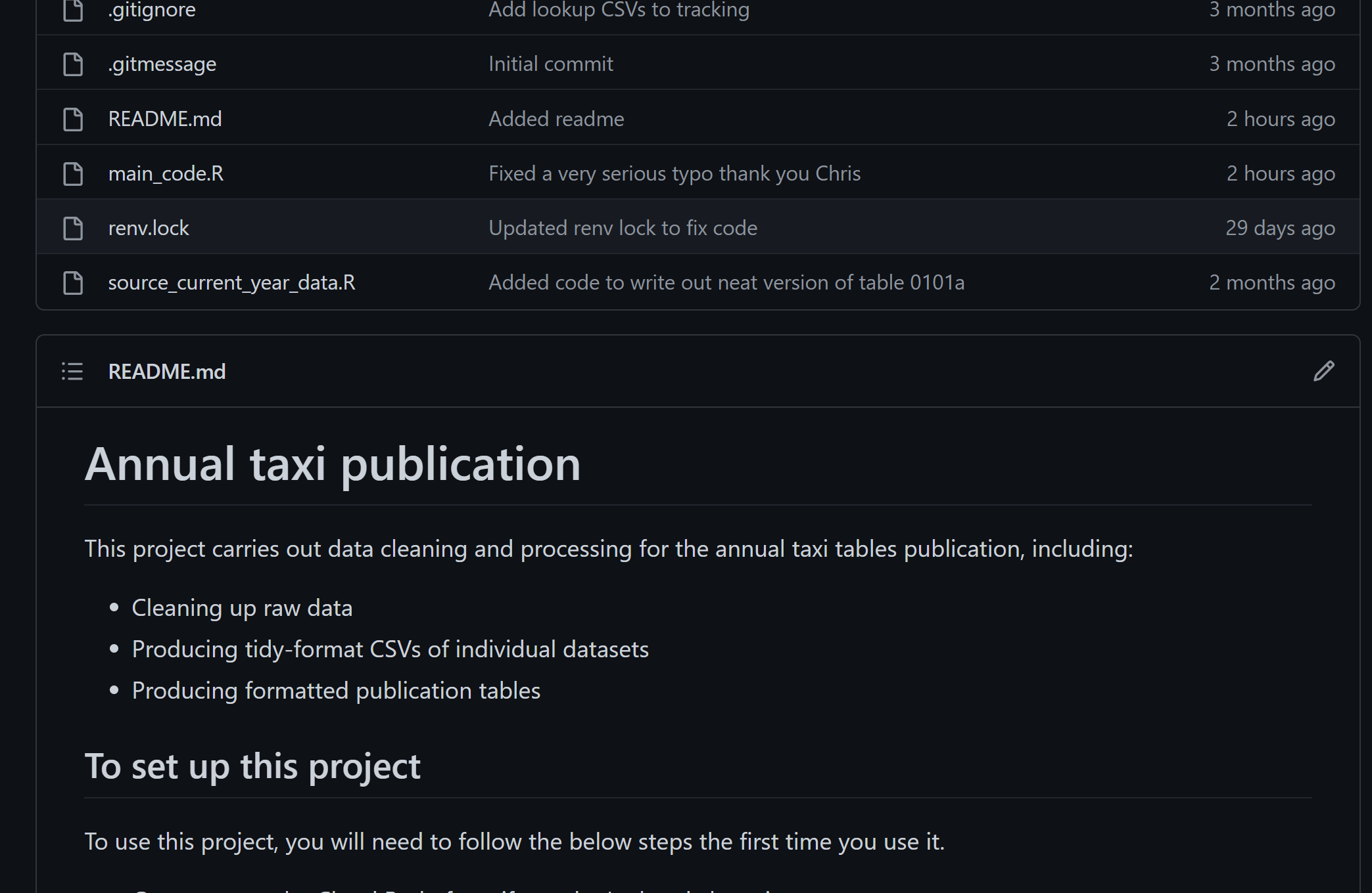
If you’re trying to find a README in a local project, search through the files in the folder for something called README; this may be a .md, .html or .Rmd file. Any of these can be opened in R, so feel free to open it and have a read.
Hopefully, the README will have told you how to use and update the code. If it’s missing, not very good, or you want more information, you can also check out the inline code comments.
2.2 Code comments
Code comments are something that almost all code will use to a greater or lesser extent, and they will be written throughout the code.
Open up any R file in the project, and have a look through for code comments. These will start with one or more hashes e.g.
#This is a code comment because it starts with hashes

value <- 4 + 5

this is evaluated as code as it does not start with any hashes

##This is also a code comment
It’s worth noting that if the file you open is a .Rmd file (an Rmarkdown file), text starting with a
#may not be a code comment, but may just be a header written in Markdown language. Check out the Rmarkdown cheat sheet to learn more about what Markdown looks like.
Good code comments should provide human-readable information about what is happening in code; not just what commands are being run, but practically what is being achieved with the data and possibly why this is happening.
Using documentation should make it simple to find the section of the code you need to change, and should even give you enough clues to work out how to change it to get the result you want. If it doesn’t, you’ll need to work that out for yourself by understanding the code!
2.3 How to tell if code isn’t doing anything
Particularly for code that isn’t version controlled and has been around for a while, it’s not that unusual to find chunks of code that don’t do anything at all. Being able to spot these makes it much easier to debug and change code.
2.3.1 Commented-out code
Commenting-out code means adding hashes # to the start of each line of code to stop it running. Any code that starts with a hash will be treated like a comment and won’t affect the output e.g.
mtcars %>%
  dplyr::select(1:3) #%>% This pipe symbol won't run
  #dplyr::filter(cyl == 4) %>% #Neither will this line of code
  dplyr::filter(cyl %in% c(6))#, 8)) # This line of code WILL run, but will only filter on cyl == 6, and ignore the 8 after the # symbol
2.3.2 Assigning vs printing
This is the most common cause for confusion for a lot of people; you’ve got a section of code that is written nicely and when you run it in isolation, it does what you’re expecting, but it doesn’t seem to change the final dataset you obtain.
This is because there are two different ways R code can run; assigning or printing.
Assigning feeds the result of your code back to a named object, using an arrow <- or sometimes (bad practice) an equals sign =, a backwards arrow -> or an assignment pipe %<>%.
#This code creates an object called a, with a value of 9
a <- 4 + 5
If there is no assignment arrow, your code will print a return in the console, but it won’t save the object to a value.
#This code just prints out the value 9 to the console
4 + 5
## [1] 9In these simple examples this seems obvious, but in complicated code it’s easy to miss:
#This code filters the dataset on the am parameter and arranges it in order
mtcars1 <- mtcars %>%
  dplyr::filter(am == 1) %>%
  dplyr::arrange(cyl)

##This section groups and summarises the previous dataset, but crucially doesn't assign it to anything! It will print in the console and nothing else
mtcars1 %>%
  dplyr::group_by(gear) %>%
  dplyr::summarise(hp_mean = mean(hp),
                   drat_mean = mean(drat),
                   count = n(),
                   qsec_mean = mean(qsec))

##This code will now return an error because it uses columns which don't exist in the assigned object, only in the printed one.

mtcars_final <- mtcars1 %>%
  dplyr::select(hp_mean, drat_mean, qsec_mean)
You can also get into similar issues if your assigned object names are subtlely different, in the below example the name of the second object has an extra underscore so again you will see an error if you run it.
#This code filters the dataset on the am parameter and arranges it in order
mtcars1 <- mtcars %>%
  dplyr::filter(am == 1) %>%
  dplyr::arrange(cyl)

##This section groups and summarises the previous dataset, and assigns to the new object mtcars_1.

mtcars_1 <- mtcars1 %>%
  dplyr::group_by(gear) %>%
  dplyr::summarise(hp_mean = mean(hp),
                   drat_mean = mean(drat),
                   count = n(),
                   qsec_mean = mean(qsec))

##This code will now return an error because it uses the old object mtcars1, not mtcars_1, where the columns don't exist.

mtcars_final <- mtcars1 %>%
  dplyr::select(hp_mean, drat_mean, qsec_mean)
If you encounter code that fails in a strange way like this, or code that is “temperamental” or needs to be run multiple times to work, it’s usually an assignment issue. Check the names and the assignments are correct for each object!
Note: There are some rarer packages where functions assign back to the original object automatically and you don’t necessarily need to assign like this; the most noteable example is data.table. It’s unlikely you will come across this, but just something to be aware of!
2.4 Understanding and changing what code is doing
One of the hardest things about working with an existing code base is understanding what it’s doing in the first place! Once you know what the current code is and isn’t doing, it’s easy to make small changes to that.
2.4.1 Libraries you should know
One of the most powerful things about R is that it has such a vast array of user-created libraries, but that wide range of choice can also make it tricky to know what libraries to use, or what libraries others are using.
The most common range of libraries you’ll come across is the tidyverse which includes a lot of the most common and easy to use packages like {dplyr}, {tidyr} and {ggplot2}. When in doubt, stick with these; and if you’re searching online for a solution to a problem don’t be afraid to add the word “tidyverse” on to your query; this will give you results that match well with your existing code and are easy for you to write and understand.
Other packages you’ll frequently come across include:
- openxlsx and other specialist reading packages: these allow you to read and write Excel files, or other unusual file types like ODS or SPSS files.
- leaflet, sf, or other mapping packages: these geospatial packages are for working with maps and geographical data.
- shiny and related packages: these are used in the dashboarding/app building world of shiny
- rmarkdown: used to create markdown reports within R
If you ever see a library name you don’t recognise, the easiest solution is to google it!
If it’s on CRAN, the first result you get can often look quite intimidating:
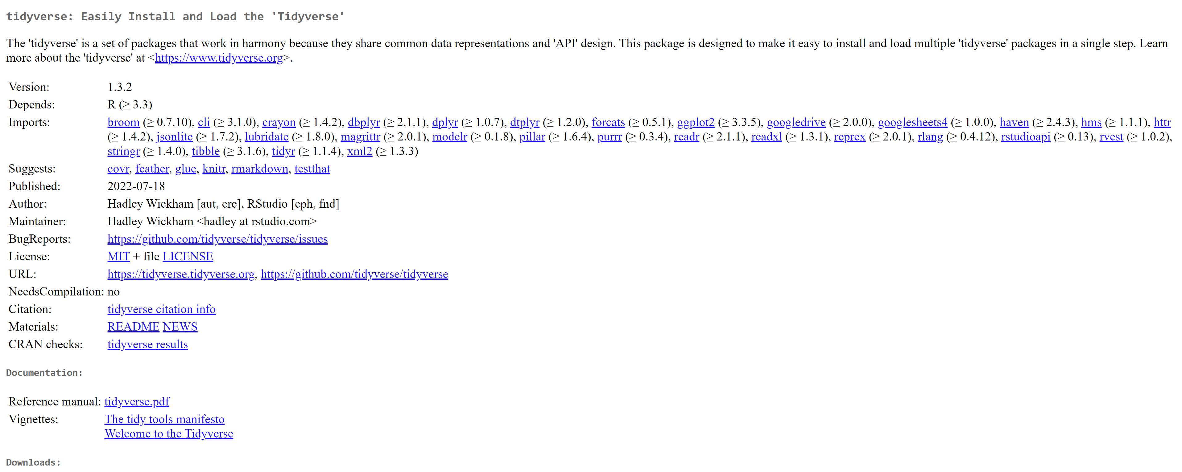
But this actually contains a lot of helpful information! Check in the documentation section to look at the reference manual, which takes you through the functions one by one, or the vignettes for examples of how to use the package. You may also find futher information by clicking on the URL links; often these take you to a dedicated package website, or a Github repo with a user-friendly README.
If a package doesn’t come up on CRAN, often it’ll be a Github or similarly hosted package, and the Github README will contain similar instructions for use.
When expanding code someone else has written, try not to add new packages unless absolutely necessary. You’ll almost always be able to achieve the same thing in multiple ways, and sticking to the packages they used makes it easier for the next person to understand the whole code base.
2.4.2 Sourcing files
You might be used to the code in a project being contained within one or more code files; you run the lines in the file, and the code there runs. However, sometimes you might notice that code runs that isn’t part of the file you’re running.
This happens through use of the source() function. This function takes a single argument (the name of an R file), and works like you’ve run all of the code inside that file at the point in the code where the source() call is made. This can be done inside of regular R files as well as Rmarkdown files.
This is a really efficient way of running projects as you can ensure your code files don’t get too long, but makes sure people are running your code in order. However, sometimes if there’s an error, it can make it tricky to work out where the error is.
You can open up any sourced file and run the code line-by-line. You can also search through an entire project for keywords using CTRL + SHIFT + F, so even if you don’t know exactly which sourced file contains the code you’re looking for, it’s easy to find.
It’s also worth noting that running source() runs the last saved version of that file; if you’re making changes and forget to save the file, running source() will give you a different result to running the code in the file directly.
2.4.3 Understanding code
When you’re faced with a large code base, it can often be really intimidating to find out what each line of code is doing just by reading it. The most simple solution is always to step through the code slowly!
This is easiest to do with code which is well-presented and makes use of pipes and the tidyverse packages (see the next chapter for details on getting your code to this state!). For example, imagine you have the code below:
gapminder %>%
  filter(continent == "Asia" & year > 1992) %>%
  group_by(country) %>%
  summarise(life_exp = mean(lifeExp))
To see what the data looks like after the first step, you can highlight the code and run it using CTRL + ENTER. Highlighting from the word “gapminder” to the end of the bracket on the row below is the equivalent of running:
##Start and end your highlight at the ** notations
** gapminder %>%
  filter(continent == "Asia" & year > 1992) ** %>%
  group_by(country) %>%
  summarise(life_exp = mean(lifeExp))

##Is the equivalent of running:
gapminder %>%
  filter(continent == "Asia" & year > 1992)
Note: make sure you don’t run the pipe (%>%) at the end of the row; this will tell R it should be expecting further code from you and it won’t return an output
If code isn’t set up in this nice, neat way, it’s usually written in a nested fashion, e.g.:
summarise(group_by(filter(gapminder, continent == "Asia" & year > 1992), country), life_exp = mean(lifeExp))If you have code like this, you can run it from the inside out! This is a bit trickier to visualise, but has the same effect:
##Start and end your highlight at the ** notation, and run using CTRL + ENTER
summarise(group_by(** filter(gapminder, continent == "Asia" & year > 1992) **, country), life_exp = mean(lifeExp))

##Is the equivalent of running:
filter(gapminder, continent == "Asia" & year > 1992)
You can just print the output of running partial code to the console, or you can treat it like any other code:
- Assign it to an object
- Use View() to examine the output in detail
- Use glimpse() or str() to check out the shape of the data
Running code one line at a time like this allows you to check when different changes occur, and insert changes of your own into the code.
2.4.4 Functions
Functions are essential for using R, and make writing code much easier. However, because they appear to function like a black box, they can make understanding someone else’s code a bit harder!
To get your head around a function, the first call is always to ask for help. Use ? in front of any function name to bring up the help files associated with it e.g. ?sum().
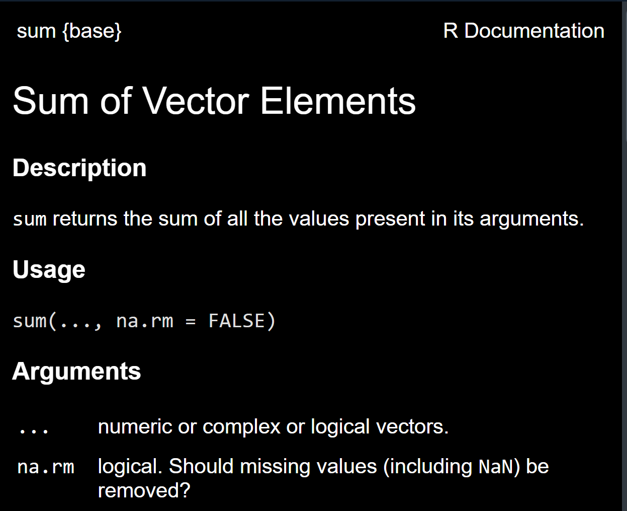
Roughly in order, help files include:
- A description of what the function actually does
- An example of how it can be used (this includes any default arguments the function has, and what those default values are)
- A list of all the arguments in the function and what they correspond to, often including what type of value the argument is expecting to receive (numeric, logical, etc).
Most people are not aware that function help files also contain example code for you to run. In the Examples section of any help file, some examples are listed; you can highlight these and use CTRL + ENTER to run them and see the function in action.
If you’re trying to debug or change the use of a function, passing it a simple dataset to check how it is working is a helpful approach. In order, you can try:
- Passing it the dataset used in the examples
- Passing it a dataset with the same structure (cols and rows) but using values from your dataset instead
- Reducing your real dataset down to just the essential columns and a few rows, and trying the function on just that
- Examining the column classes and types to see which differ between your dataset and the test dataset.
2.4.4.1 User-defined functions
Sometimes in your code, you may also come across use of a user-defined function; these are functions that don’t come from a package, and are instead defined and used within the same code base.
They’ll be defined in the code in the following way:
function_name <- function(function, arguments, here){

  function_code_in_here
}
Remember you can use CTRL + SHIFT + F to search through a whole project and find where the function is first defined in the code base to check it doesn’t come from a package.
If you’re lucky, they will be documented in exactly the same way as a package function, and you’ll be able to use the ? symbol to call up the associated helpfile.
If not, you can test and debug them in a similar way to package functions, feeding them test data to understand how they work.
You can also “step-into” a user defined function to run it line-by-line, like you would for any non-function code. You can do this pretty easily by assigning the arguments as objects, then running the code inside the curly brackets {} one line at a time to see what it does:
my_fun <- function(x, y, z){

  if(x == 2){

    y * z + x

  } else{
    x <- x ^ 2

    y * z * x
  }


}
I can assign default values to x, y and z by running x = 1, y = 2, z = 1 in the console, and then running the code inside the function in a stepwise way.
2.5 Warnings vs errors vs messages
The way that R communicates with users can often be quite confusing if you’re not used to it, and quite frequently new users aren’t clear exactly what it going on when they run code. Whenever it runs code, R will communicate information about that code to you in the console.
There are a few different options:
- No message at all, just a
>Congratulations, your code worked! R is set up to “fail loudly, pass quietly” so if you get no message at all it means that there were no problems. - Error: (some text here) Your code has encountered a breaking change; it has exited the process and will not produce an output other than that error. It’s easy to see error messages as an “oh no, it’s broken” alert, but in R they usually provide a lot of very helpful information. Check out the bugfixing section above to see how to get the most from error messages.
- Warning: (some text here) Your code has run, but has something important it wants to tell you. Crucially, warnings can be a big problem, or they can be completely fine, it doesn’t necessarily mean there’s something wrong with your code. An example:
as.numeric(c("a", 1, "2"))## Warning: NAs introduced by coercion## [1] NA 1 2Notice that above, you get a warning saying that running the as.numeric() function has converted some values to NAs. This is totally expected, the letter “a” can’t be converted to a numerical value, so it will be turned into an NA, but the warning message can make you assume that the code hasn’t run at all.
* Message Any text that doesn’t start with Warning: or Error: is just a message. It’s telling you information about the process that’s running, but there’s no suggestion that the code isn’t working or is doing anything unusual. Do check your messages carefully in case what it’s reported isn’t what you expect the code to be doing though!